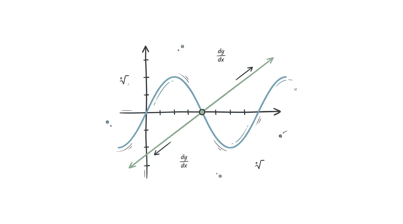
In Cartesian geometry, a real-valued 2D function y=f(x) maps an independent scalar variable x∈R to a unique dependent output y∈R. The resulting graph represents the continuous set of ordered pairs (x,f(x)) embedded within a 2D plane.
Below is an interactive 2D Graph Plotter. Use the dropdown preset selector to analyze polynomial functions, trigonometric waves, Gaussian bell curves, or implicit circles. Hover over any region on the graph to inspect exact (x,y) coordinate evaluation and instantaneous derivative tangent slope f′(x):
Interactive 2D Function Plotter & Tangent Slope Engine
y = sin(x)y = cos(x)
Curves:
Hover cursor over graph to inspect coordinates
2. Mathematical Analysis of 2D Curves
Derivative Slopes & Tangent Lines
The instantaneous rate of change (slope of the tangent line) at point (x0,f(x0)) is given by the First Derivative:
m=f′(x0)=Δx→0limΔxf(x0+Δx)−f(x0)
The explicit point-slope equation of the tangent line is:
y−f(x0)=f′(x0)⋅(x−x0)
Local Extrema & Critical Points
A continuous function achieves local maxima or minima at critical points where f′(x)=0 or where f′(x) is undefined.
First Derivative Test: If f′(x) changes sign from positive to negative at x0, f(x0) is a local maximum.
Second Derivative Test:
If f′′(x0)>0, the curve is concave up (local minimum).
If f′′(x0)<0, the curve is concave down (local maximum).
3. Implicit 2D Curves (F(x,y)=0)
Not all 2D curves can be expressed as explicit functions y=f(x). Implicit equations constrain both variables simultaneously:
x2+y2=R2(Circle of radius R)
Using Implicit Differentiation, the tangent slope dxdy is derived by taking the derivative with respect to x on both sides: