Deep Learning Foundations: Gradient Descent, Multilayer Backpropagation Calculus & Loss Optimization

Artificial Neural Networks (ANNs) form the computational backbone of contemporary artificial intelligence, powering everything from computer vision models to large language transformers. At its core, training a neural network is a high-dimensional mathematical optimization problem: finding a point in weight space $\mathbf{W} \in \mathbb{R}^d$ that minimizes an empirical loss function $\mathcal{L}(\mathbf{W})$.

In this exhaustive analytical guide, we explore the complete mathematical engine driving deep learning: vectorized forward propagation, loss surface geometry, multivariate vector calculus, complete multilayer backpropagation step-by-step derivations, and modern adaptive gradient descent algorithms.

1. Mathematical Foundations & Vectorized Forward Pass

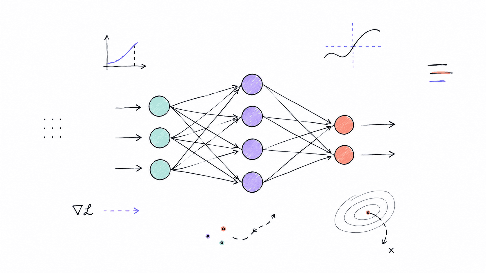
An artificial neural network consists of interconnected layers of artificial neurons. Let $L$ denote the total number of layers in the network, where layer $l = 0$ is the input layer and layer $l = L$ is the output layer.

$l \in \{0, 1, 2, \dots, L\}$

Vectorized Layer Transformation

For any hidden layer $l$, the linear sum vector $\mathbf{z}^{(l)} \in \mathbb{R}^{n_l}$ is calculated by multiplying the weight matrix $\mathbf{W}^{(l)} \in \mathbb{R}^{n_l \times n_{l-1}}$ with the activation vector from the previous layer $\mathbf{a}^{(l-1)} \in \mathbb{R}^{n_{l-1}}$, plus the bias vector $\mathbf{b}^{(l)} \in \mathbb{R}^{n_l}$:

$\mathbf{z}^{(l)} = \mathbf{W}^{(l)} \mathbf{a}^{(l-1)} + \mathbf{b}^{(l)}$

The activation vector $\mathbf{a}^{(l)}$ is subsequently produced by applying an element-wise non-linear activation function $\sigma(\cdot)$:

$\mathbf{a}^{(l)} = \sigma\left(\mathbf{z}^{(l)}\right)$

$\text{where } \mathbf{a}^{(0)} = \mathbf{x} \quad (\text{the input feature vector})$

Activation Functions & Nonlinearity

Without non-linear activation functions, a deep neural network—regardless of its depth—collapses into a single linear matrix transformation:

$\mathbf{y} = \mathbf{W}^{(L)} \mathbf{W}^{(L-1)} \dots \mathbf{W}^{(1)} \mathbf{x} = \mathbf{W}_{\text{effective}} \mathbf{x}$

Non-linear activation functions allow neural networks to approximate arbitrary continuous functions (The Universal Approximation Theorem).

1. Sigmoid Activation Function

$\sigma(z) = \frac{1}{1 + e^{-z}}, \quad \sigma'(z) = \sigma(z)\left(1 - \sigma(z)\right)$

2. Rectified Linear Unit (ReLU)

$\text{ReLU}(z) = \max(0, z), \quad \text{ReLU}'(z) = \begin{cases} 1 & z > 0 \\ 0 & z \le 0 \end{cases}$

3. Hyperbolic Tangent (Tanh)

$\tanh(z) = \frac{e^z - e^{-z}}{e^z + e^{-z}}, \quad \tanh'(z) = 1 - \tanh^2(z)$

2. Loss Landscapes & Optimization Objectives

To train a neural network, we quantify the discrepancy between network predictions $\mathbf{\hat{y}} = \mathbf{a}^{(L)}$ and true target labels $\mathbf{y}$ using a scalar loss function $\mathcal{L}$.

Mean Squared Error (MSE) Loss

Used predominantly in regression tasks:

$\mathcal{L}_{\text{MSE}}(\mathbf{y}, \mathbf{\hat{y}}) = \frac{1}{2} \|\mathbf{y} - \mathbf{\hat{y}}\|_2^2 = \frac{1}{2} \sum_{k=1}^{K} (y_k - \hat{y}_k)^2$

Binary Cross-Entropy (BCE) Loss

Used in binary classification tasks:

$\mathcal{L}_{\text{BCE}}(y, \hat{y}) = - \Big[ y \log(\hat{y}) + (1 - y) \log(1 - \hat{y}) \Big]$

The Loss Surface Manifold

The loss function $\mathcal{L}(\mathbf{W})$ defines a scalar field over high-dimensional weight space. For simple quadratic loss functions, the loss surface is convex (a 3D bowl shape), guaranteeing a global minimum:

$\mathcal{L}(w_1, w_2) = w_1^2 + w_2^2$

In deep multi-layer networks, however, non-linear activations render the loss surface non-convex, featuring local minima, high-dimensional saddle points, and flat plateaus:

$\mathcal{L}(w_1, w_2) = w_1^2 - w_2^2 + 0.5 \cdot \sin(3 w_1) \cos(3 w_2)$

3. Multivariable Vector Calculus & Gradient Descent

The gradient vector $\nabla_{\mathbf{W}} \mathcal{L}$ collects all partial derivatives of the scalar loss $\mathcal{L}$ with respect to every weight parameter:

$\nabla_{\mathbf{W}} \mathcal{L} = \left[ \frac{\partial \mathcal{L}}{\partial w_1}, \frac{\partial \mathcal{L}}{\partial w_2}, \dots, \frac{\partial \mathcal{L}}{\partial w_d} \right]^T$

The gradient vector $\nabla_{\mathbf{W}} \mathcal{L}$ points in the direction of maximum rate of increase of the loss function. Consequently, to minimize the loss, we step in the opposite direction of the gradient:

$\Delta \mathbf{W} = - \eta \nabla_{\mathbf{W}} \mathcal{L}$

where $\eta > 0$ represents the learning rate hyperparameter.

Gradient Descent Iterative Update Rule

$\mathbf{W}^{(t+1)} = \mathbf{W}^{(t)} - \eta \nabla_{\mathbf{W}} \mathcal{L}\left(\mathbf{W}^{(t)}\right)$

$\mathbf{b}^{(t+1)} = \mathbf{b}^{(t)} - \eta \nabla_{\mathbf{b}} \mathcal{L}\left(\mathbf{b}^{(t)}\right)$

4. Multilayer Backpropagation Algorithm: Step-by-Step Calculus Derivation

Backpropagation (backward propagation of errors) is an efficient application of the multivariable Chain Rule of Calculus used to evaluate gradients $\frac{\partial \mathcal{L}}{\partial \mathbf{W}^{(l)}}$ and $\frac{\partial \mathcal{L}}{\partial \mathbf{b}^{(l)}}$ across all layers $l \in \{1, \dots, L\}$.

Let us define the error delta vector $\delta^{(l)} \in \mathbb{R}^{n_l}$ for layer $l$ as the partial derivative of loss with respect to pre-activation linear sums $\mathbf{z}^{(l)}$:

$\delta^{(l)} \equiv \frac{\partial \mathcal{L}}{\partial \mathbf{z}^{(l)}}$

5. Advanced Optimization Algorithms

Plain Stochastic Gradient Descent (SGD) can oscillate in ravines or stall at saddle points. Modern deep learning relies on adaptive momentum-based optimization algorithms.

1. SGD with Momentum

Accumulates an exponentially decaying moving average of past gradients to accelerate along persistent directions:

$\mathbf{v}_t = \beta \mathbf{v}_{t-1} + (1 - \beta) \mathbf{g}_t$

$\mathbf{W}_{t+1} = \mathbf{W}_t - \eta \mathbf{v}_t$

2. Adam (Adaptive Moment Estimation)

Combines momentum (first moment $m_t$) and RMSprop (second uncentered moment $v_t$) with bias correction:

$m_t = \beta_1 m_{t-1} + (1 - \beta_1) g_t, \quad v_t = \beta_2 v_{t-1} + (1 - \beta_2) g_t^2$

$\hat{m}_t = \frac{m_t}{1 - \beta_1^t}, \quad \hat{v}_t = \frac{v_t}{1 - \beta_2^t}$

$\mathbf{W}_{t+1} = \mathbf{W}_t - \frac{\eta}{\sqrt{\hat{v}_t} + \epsilon} \hat{m}_t$

6. Interactive Deep Learning Engine & Real-Time Activation Explorer

Below is an interactive deep neural network engine. You can tweak layer activation functions, adjust learning rate $\eta$, execute single backpropagation steps, or run auto-training loops to observe real-time loss convergence $L(\mathbf{W})$:

Summary & Architectural Insights

1. Forward Propagation: Computes linear transformations $\mathbf{z}^{(l)} = \mathbf{W}^{(l)} \mathbf{a}^{(l-1)} + \mathbf{b}^{(l)}$ followed by non-linear activations $\mathbf{a}^{(l)} = \sigma(\mathbf{z}^{(l)})$.
2. Loss Surfaces: Non-convex loss manifolds in high dimensions contain saddle points and local minima, requiring momentum and adaptive learning rates.
3. Backpropagation: Calculates error deltas $\delta^{(l)} = ((\mathbf{W}^{(l+1)})^T \delta^{(l+1)}) \odot \sigma'(\mathbf{z}^{(l)})$ from output to input via multivariable chain rule.
4. Gradient Updates: Weights and biases adapt proportionally to $\eta \cdot \delta^{(l)} (\mathbf{a}^{(l-1)})^T$.