How Neural Networks Learn: Activation Functions, Weight Initialization & Optimization Dynamics

Without non-linear activation functions, a neural network with 100 hidden layers is mathematically equivalent to a single linear regression model. Learning happens at the intersection of non-linear transformations, proper weight variance preservation, and adaptive gradient optimization.

Training deep neural networks requires coordinating three fundamental building blocks: non-linear activation functions, variance-preserving weight initializations, and adaptive first/second-order optimization algorithms.

1. Activation Functions: Introducing Non-Linearity

Without activation functions, matrix multiplications accumulate into a single linear map:

$\mathbf{y} = \mathbf{W}_3 (\mathbf{W}_2 (\mathbf{W}_1 \mathbf{x} + \mathbf{b}_1) + \mathbf{b}_2) + \mathbf{b}_3 = \mathbf{W}_{net} \mathbf{x} + \mathbf{b}_{net}$

Activation functions $\sigma(z)$ break this linearity, enabling networks to approximate arbitrary continuous functions (The Universal Approximation Theorem).

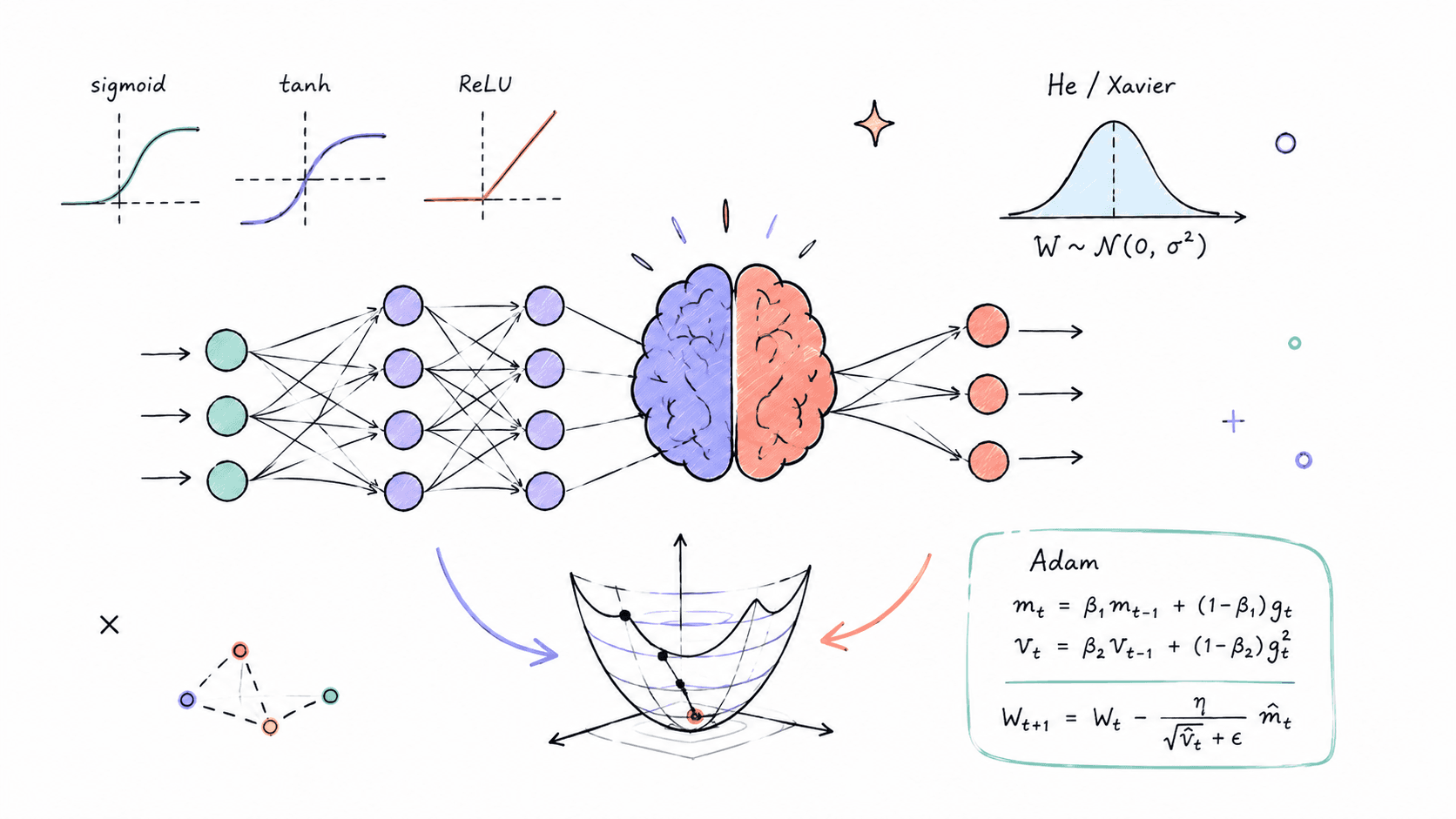
Classic Activation Landscapes

1. Sigmoid: $\sigma(z) = \frac{1}{1 + e^{-z}}$ (vanishes gradients for $|z| > 4$)
2. Hyperbolic Tangent (Tanh): $\tanh(z) = \frac{e^z - e^{-z}}{e^z + e^{-z}}$ (zero-centered)
3. Rectified Linear Unit (ReLU): $f(z) = \max(0, z)$ (prevents vanishing gradients for $z > 0$)

2. Weight Initialization: Preserving Variance Across Layers

If weight matrices are initialized too large, activations explode ($1.5^{100} \to \infty$). If initialized too small, activations collapse to zero ($0.5^{100} \to 0$).

To prevent vanishing and exploding gradients during forward and backward passes, we initialize weights so that variance is preserved from layer to layer:

$\text{Var}(z^{(l)}) = \text{Var}(a^{(l-1)})$

Xavier (Glorot) Initialization (for Sigmoid / Tanh)

For a layer with $n_{\text{in}}$ inputs and $n_{\text{out}}$ outputs, weights are drawn from a normal distribution with variance:

$\mathbf{W}_{i,j} \sim \mathcal{N}\left(0, \, \frac{2}{n_{\text{in}} + n_{\text{out}}}\right)$

He (Kaiming) Initialization (for ReLU)

Because ReLU zero-out half of all negative inputs (halving the variance), He initialization compensates by doubling the variance:

$\mathbf{W}_{i,j} \sim \mathcal{N}\left(0, \, \frac{2}{n_{\text{in}}}\right)$

3. Interactive Neural Learning Lab

Simulate forward activation flow, loss computation, backpropagation error deltas, and real-time weight matrix updates using the interactive laboratory below:

4. Adaptive Optimization Algorithms

Standard Stochastic Gradient Descent (SGD) updates weights along the negative gradient direction:

$\mathbf{W}_{t+1} = \mathbf{W}_t - \eta \cdot \nabla_{\mathbf{W}} \mathcal{L}(\mathbf{W}_t)$

In non-convex, high-dimensional loss landscapes with ravines and saddle points, modern adaptive optimizers accelerate convergence:

Adam (Adaptive Moment Estimation)

Adam maintains moving averages of both the first moment (mean $m_t$) and second moment (uncentered variance $v_t$) of gradients:

$m_t = \beta_1 m_{t-1} + (1 - \beta_1) g_t$

$v_t = \beta_2 v_{t-1} + (1 - \beta_2) g_t^2$

With bias correction:

$\hat{m}_t = \frac{m_t}{1 - \beta_1^t}, \quad \hat{v}_t = \frac{v_t}{1 - \beta_2^t}$

$\mathbf{W}_{t+1} = \mathbf{W}_t - \frac{\eta}{\sqrt{\hat{v}_t} + \epsilon} \hat{m}_t$

Summary

• Activation Functions: Use ReLU or LeakyReLU by default for hidden layers to prevent vanishing gradients.
• Initialization: Match activation functions with appropriate initializers (He for ReLU, Xavier for Tanh/Sigmoid).
• Optimization: Use Adam ($\eta = 10^{-3}$) for rapid prototyping and non-convex landscapes, or SGD with Momentum ($\beta = 0.9$) for optimal generalization on vision tasks.