Integral calculus is one of the foundational pillars of modern mathematical physics, continuous probability theory, and machine learning. At its core, integration measures cumulative quantity—whether computing areas under curves, volumes of higher-dimensional manifolds, or total probability densities.
1. The Fundamental Definition: Riemann Sums & Limit Processes
The definite integral of a real-valued function over a closed interval is defined as the limit of a Riemann sum as the mesh size of the partition approaches zero:
Where:
- is a partition of with and .
- represents the width of the -th subinterval.
- is an arbitrary sample evaluation point.
If this limit exists independently of the choice of partition and sample points , the function is declared Riemann integrable.
2. Fundamental Theorem of Calculus (FTC)
The Fundamental Theorem of Calculus bridges differential operator rates of change with cumulative integral accumulation.
Part 1: Accumulation Function Derivative
If is continuous on , then the accumulation function is continuous on , differentiable on , and satisfies:
Part 2: Evaluation Theorem
If is any antiderivative of such that , then:
3. Advanced Integration Techniques & Analytical Solutions
Integration by Parts
Derived directly from the differential product rule :
For example, integrating :
The Gaussian Integral (Euler-Poisson Integral)
One of the most essential integrals in statistics and quantum mechanics is the Gaussian probability integral:
Handwritten Engineering Computation Pad
4. Numerical Quadrature Implementations
When analytical antiderivatives do not exist (e.g. ), numerical quadrature algorithms estimate the definite integral.
1import numpy as np2from scipy.integrate import quad3import sympy as sp45# 1. Analytical Symbolic Integration using SymPy6x = sp.Symbol('x')7f_expr = sp.exp(-x**2)8exact_indefinite = sp.integrate(f_expr, x)9print(f"[SymPy] Indefinite Integral of e^(-x^2): {exact_indefinite}")1011# 2. Numerical Integration using Composite Simpson's 1/3 Rule12def simpsons_rule(f, a, b, n=1000):13 if n % 2 != 0:14 n += 1 # n must be even for Simpson's rule15 x_pts = np.linspace(a, b, n + 1)16 h = (b - a) / n17 y_pts = f(x_pts)1819 integral = (h / 3) * (y_pts[0] + 4 * np.sum(y_pts[1:-1:2]) + 2 * np.sum(y_pts[2:-2:2]) + y_pts[-1])20 return integral2122# Evaluate Gaussian integral from -5 to +523gaussian = lambda x: np.exp(-x**2)24approx = simpsons_rule(gaussian, -5.0, 5.0, n=10000)25exact_scipy, err = quad(gaussian, -np.inf, np.inf)2627print(f"[Simpson's 1/3] Computed Integral: {approx:.8f}")28print(f"[SciPy Quad] Exact Integral: {exact_scipy:.8f} (Error: {err:.2e})")29print(f"[Theoretical] sqrt(pi): {np.sqrt(np.pi):.8f}")
5. Summary Equation Reference Table
| Formula Name | Analytical Expression | Primary Use Case |
|---|---|---|
| Definite Integral | Computing net accumulated area | |
| Gaussian Integral | Normal probability density normalization | |
| Integration by Parts | Products of transcendental functions | |
| Laplace Transform | Differential equation domain transformation |